Indirect lighting through irradiance probes: Theory and practice

This articles was made as part of an assignment during my studies at BUas (Breda University of applied sciences)

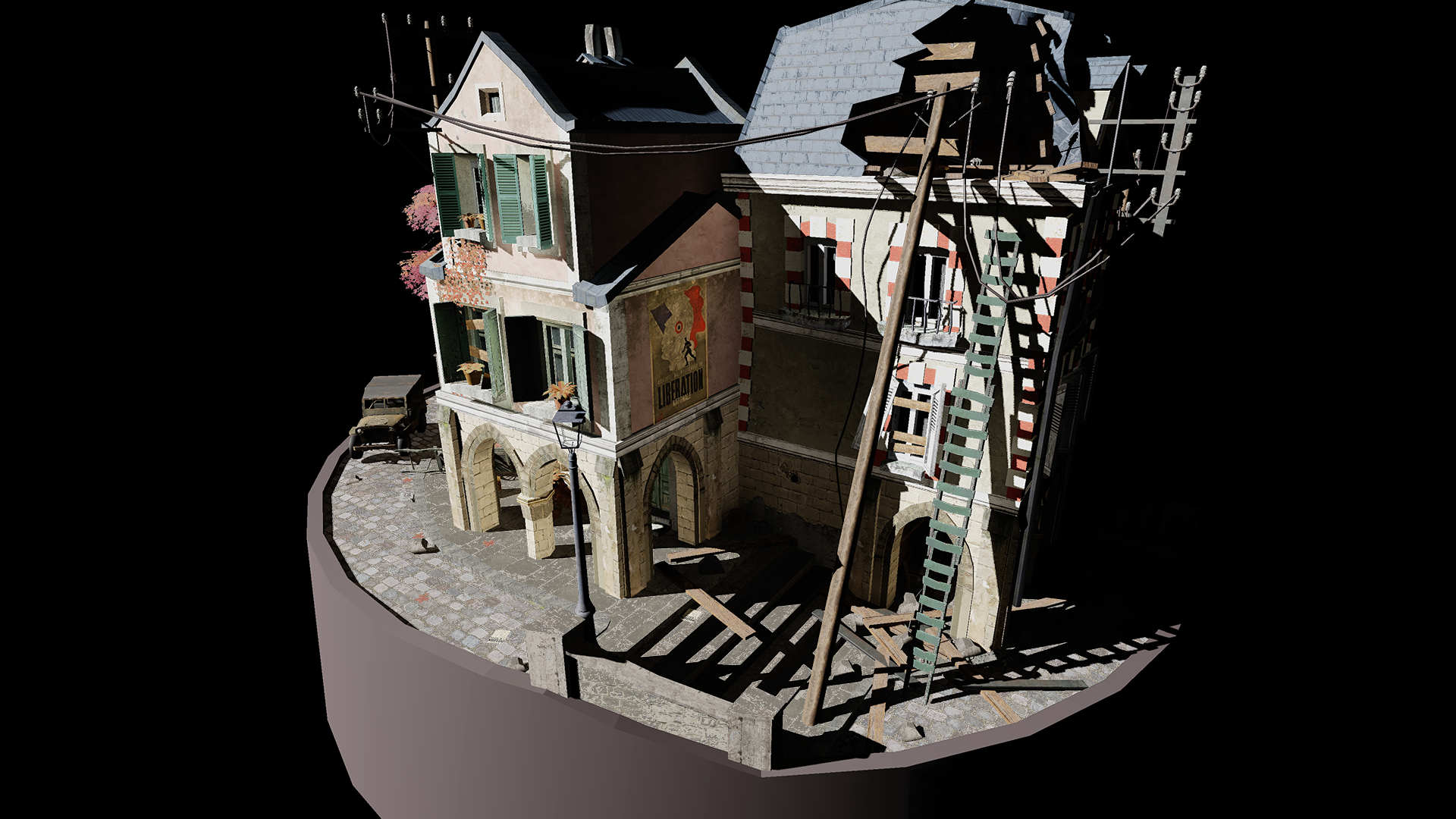
Exposure corrected final result (simulating shadow and highlight exposure correction through masking in photoshop see for more info)

Indirect lighting through irradiance probes: Theory and practice
Table of contents
Introduction - Why indirect illumination?
Theory
Implementation
Exposure correction explanation
Sources

Introduction

I am currently enrolled at Breda University of Applied Sciences as a 2nd year programming student, this blog post was written as part of my grading for the given feature I had to implement. I have written this post to condense the research and implementation into a single readable format. As this post expands beyond what I will be graded for I hope you will be able to learn and gain some insights from this article.

Why indirect illumination?

This school project of mine needed me to learn the necessary skills for a chosen industry position. I chose the position of graphics programmer at Naughty Dog and oriented my project around approximating indirect illumination. As I learned from Naughty Dog at Siggraph 2020[1] they use a probe based lighting scheme for indirect illumination so this is what I based my implementation on.

Theory

Abstract

The problem we’re solving here is approximating indirect illumination in a way that better simulates light bouncing through the scene instead of a flat ambient term. Tons of research has already been poured into this problem. I have assembled an implementation based on several different research papers and implementations (see sources)

Comparison between flat ambient term and probe based indirect illumination

Solving the irradiance question

Irradiance data can roughly be explained as the incoming light from all possible directions, so how de we generally solve this unknown?

Since calculating irradiance means integrating the light coming from an infinite possibility of directions over a hemisphere it is infeasible to expect any answer, let alone in real-time on consumer hardware. This means we have to approximate the irradiance using something like a Riemann sum, this process of discretization generally returns results that are more than good enough for real-time purposes, this yield us with the following equation we have to compute:

\[L_o(p, \phi_o, \theta_o) = k_d {c \over \pi} \int_{\phi=0}^{2\pi} \int_{\theta=0}^{\frac{1}{2}\pi} L_i(p, \phi_i, \theta_i) \cos(\theta) \sin(theta) d\phi d\theta\]

In polar coordinates[5]

\[L_o(p, \phi_o, \theta_o) = k_d {c\pi \over n1n2} \sum_{\phi = 0}^{n1} \sum_{\theta=0}^{n2} L_i(p, \phi_i, \theta_i) \cos(\theta) \sin(theta) d\phi d\theta\]

As a Riemann-sum approximation [5] with n1 and n2 discrete samples

Where L_i is the incoming light and L_o the irradiance

We can then use this equation to compute the irradiance and store this in several ways, Like cubemaps in the classic IBL implementation or spherical harmonics for a more efficient use of memory

Storing of irradiance values in a cubemap, Each pixel represents the irradiance for a given normal

Populating probes in a scene

Ideally, we would calculate the irradiance for a given point and it’s normal in the scene, but, since solving the equation in Solving the irradiance question in a real-time application is infeasible we have to rely on an approximation. In my implementation I use something called a probe (diffuse probe, irradiance probe, IBL probe, light probe, e.t.c.), that captures the irradiance at a given point in the scene.
Luckily diffuse irradiance data depening on the density of placements doesn’t vary that much spatially so generally these approximations return results that are plausible enough.

Some options to consider when placing probes in the scene

Placing on a regular grid
Sparse placement
Hand placing probes

When placing these probes keep in mind how they will be interpolated, by using the regular grid we use a trilinear interpolation function, the same interpolation techniques will carry over to something like a sparse grid, but depending on how you place the probes within your own data structure you might need to use a more complex interpolation method.

Implementation

The implemenation of this requires some rewriting in pseudo code as it was fully created on a Playstation 5®. With this in mind I hope there is still something to take away from reading this.

High-level overview

The high level overview of the implementation goes as follows:

Create a regular grid containing the scene
For each point on the grid:
- Draw a cubemap
- Convert this cubemap to spherical harmonics
When drawing:
- Get the world space postion and the normal for given pixel/fragment
- With a lookup function find the eight corners of the grid cell overlapping the position
- trilinearly interpolate between the eight probes, discarding the probes that are behind the surface normal
- Add this to the final radiance (replacing the ‘ambient’ term)

Reducing the irradiance memory print

As alluded to in the theoretical side of this article we use 2nd order spherical harmonics for storing the irradiance[6]. This reduces the memory footprint for diffuse data to 9 3-component vectors. or in shader language.

struct SH9Irradiance
{
    float3 band0_0;
    float3 band1_n1, band1_n0, band1_p1;
    float3 band2_n2, band2_n1, band2_0, band2_p1, band2_p2;
};

A single probe is then represented like this

struct Probe
{
    SH9Irradiance IrradianceCoefficients;
    float3 Position;
}

For any given normal we can generate the coefficients for each order and band using the following function:

SH9 GenSHCoefficients(float3 normal)
{
	sh::SH9 result;

	result.band0_0 = 0.282095f;

	result.band1_n1 = 0.488603f * normal.y;
	result.band1_0 = 0.488603f * normal.z;
	result.band1_p1 = 0.488603f * normal.x;

	result.band2_n2 = 1.092548f * normal.x * normal.y;
	result.band2_n1 = 1.092548f * normal.y * normal.z;
	result.band2_0 = 0.315392f * (3 * normal.z * normal.z - 1.0f);
	result.band2_p1 = 1.092548f * normal.x * normal.z;
	result.band2_p2 = 0.54627f * (normal.x * normal.x - normal.y * normal.y);

	return result;
}

Where SH9 is a struct containing 9 scalar coefficients.

Retrieving the irradiance signal can then be computed as follows

float3 CalcSHIrradiance(float3 normal, SH9Irradiance irrCoeff)
{
	const float A0 = 3.141593f;
	const float A1 = 2.094395f;
	const float A2 = 0.785398f;

	SH9 coefficients = GenSHCoefficients(normal);

	return
		irrCoeff.band0_0 * coefficients.band0_0 * A0 +
		irrCoeff.band1_n1 * coefficients.band1_n1 * A1 +
		irrCoeff.band1_0 * coefficients.band1_0 * A1 +
		irrCoeff.band1_p1 * coefficients.band1_p1 * A1 +
		irrCoeff.band2_n2 * coefficients.band2_n2 * A2 +
		irrCoeff.band2_n1 * coefficients.band2_n1 * A2 +
		irrCoeff.band2_0 * coefficients.band2_0 * A2 +
		irrCoeff.band2_p1 * coefficients.band2_p1 * A2 +
		irrCoeff.band2_p2 * coefficients.band2_p2 * A2;
}

The encoding of irradiance signals into these harmonics will be displayed in the section From position to irradiance probe.

From position to irradiance probe

The pipeline for baking probes consist of a two step process:

Generate a cubemap
Use this cubemap to compute spherical harmonics

As I showed in Solving the irradiance question we can compute the irradiance integral for a cubemap by taking samples over a hemisphere for each pixel in the cubemap, We essentially do the same thing with spherical harmonics but we calculate the coefficients for different bands per pixel’s normal and add these together weighted by the differential solid angle of the pixel. As the total weight should be 4π[7][8] we normalize the weight by dividing by weightSum to make sure we apply a correct correction factor.

In a shader language:

[NumThreads(1, 1, 1)]
void main(uint3 DTid : SV_DISPATCH_THREAD_ID)
{
	uint index = DTid.x;

	SH9Irradiance irrOut = {};

	float weight, weightSum = 0.0f;
	for(uint face = 0; face < 6; face++)
	{
		for(uint x = 0; x < Resolution; x++)
		{
			for(uint y = 0; y < Resolution; y++)
			{
				float u = (x + 0.5f) / (float)Resolution;
				float v = (y + 0.5f) / (float)Resolution;
				u = u * 2.0f - 1.0f;
				v = v * 2.0f - 1.0f;
	
				float temp = 1.0f + u*u + v*v;
				weight = 4.0f/(sqrt(temp) * temp);
	
				float3 normal = GetCubefaceSamplingVector((int)face, float2(u, v));

				float3 irradiance = Cubemaps[index].Sample(sampler, normal).rgb;
				irrOut += GenerateIrradianceCoefficientsFromNormal(normal, irradiance) * weight;

				weightSum += weight;
			}
		}
	}

	irrOut *= (4.0f * PI) / weightSum;

	srtinst.Probes[index].IrradianceCoefficients = irrOut;
}

Indexing into your grid

For my implementation I index into individual grid cells using the fragment’s world space position.

Rendering

Eventually all this work leads to a relatively minor addition/replacement in the shader responsible for lighting your scene.


// Direct light calculations...

radiance += GetIrradiance(WSPosition, normal);

// Preparing for output...

Taking this a step further

Alternative features that can be implemented to improve/enhance the algorithm. Serving as inspiration to the reader as well as a list for myself to implement outside of what the 7 weeks of school work allowed me to do

Using a ray-tracer to get radiance values
Currently we generate a cubemap per probe and sample the radiance as a pixel in the texture. We could also spawn some rays per probe and use these radiance values to compute the harmonics.This process is very similair to what Nvidia uses in their real-time hardware accelerated ray-tracing global illumination algorithm[2]
Encoding visibility
The implementation only naively discards probes based on a surface normal test. This is far from sufficient in reducing light leaks. We can encode depth information in a 2d texture that maps the normals of a sphere to an unfolded octahedron[3]. Eliminating many cases where a probe is inside geometry.
Screen space ambient occlusion
To better embed objects in the scene screen space ambient occlusion is a great way to create a cohesion between objects close together.
Reflections
The implementation currently only supports diffuse irradiance data. A nice addition to handle more complex scenes would be a way to handle reflections. I’ll list several options here:
- Stochastic screen space reflections[4]
- Raytraced reflections
- Automatic or manually placed reflection probes

Exposure correction explanation

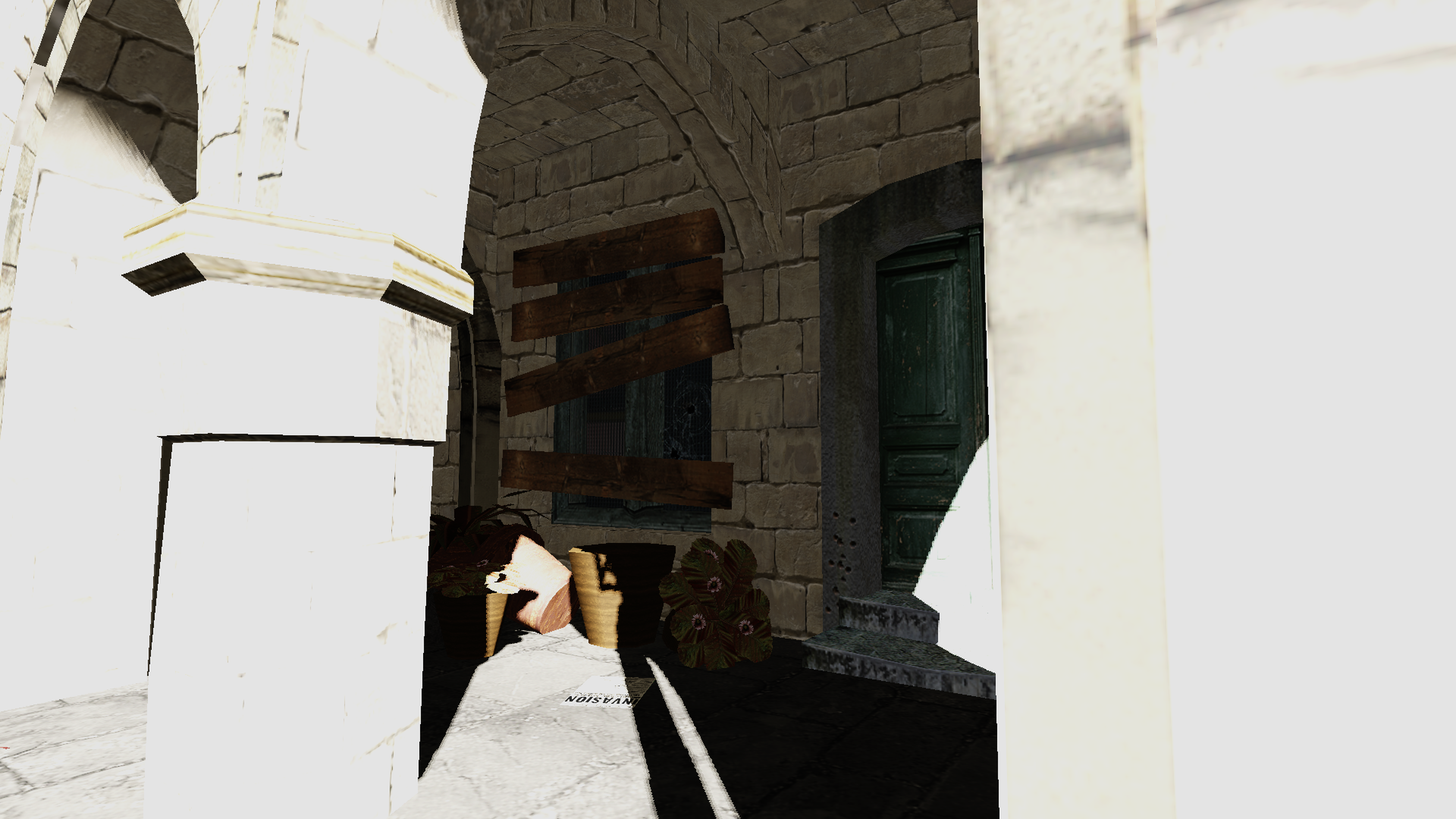
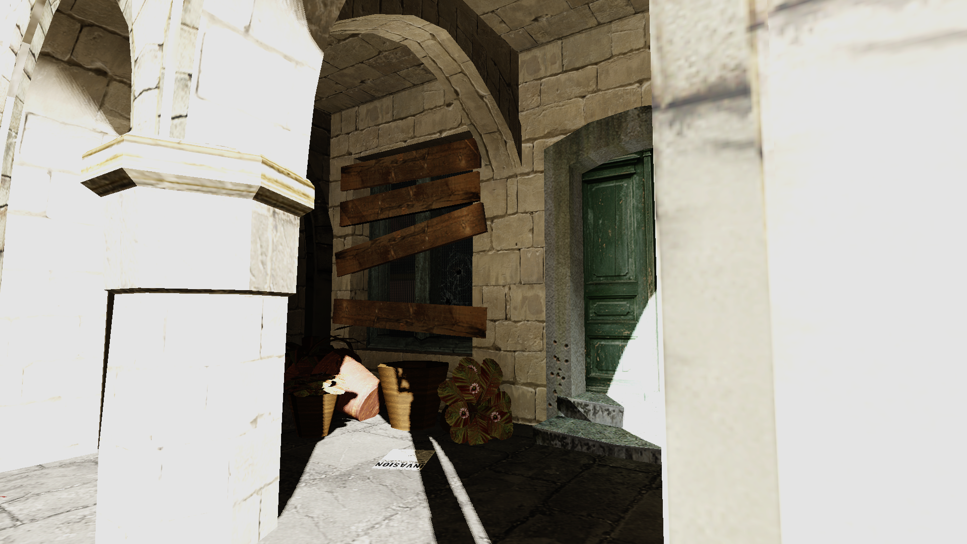
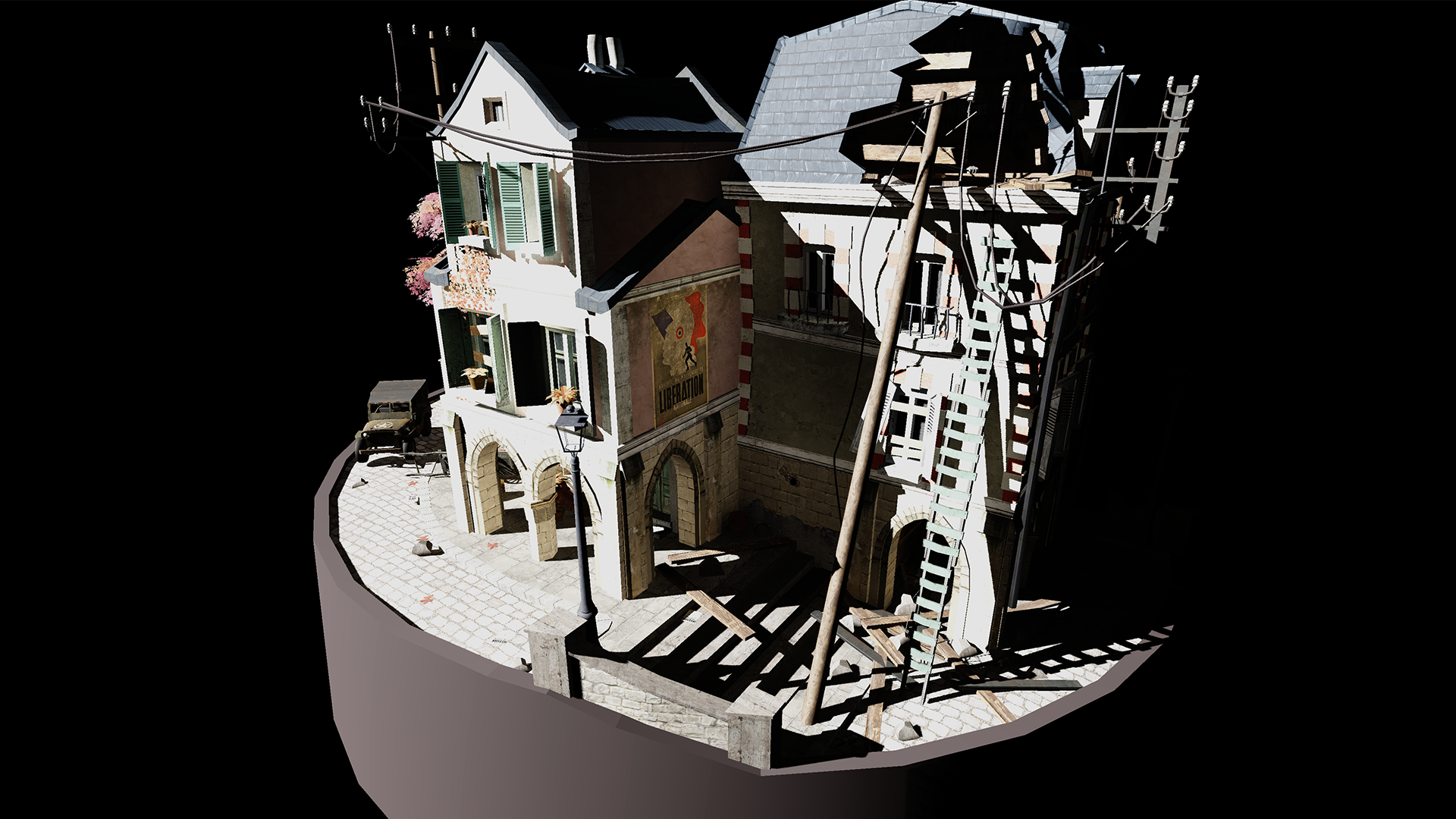
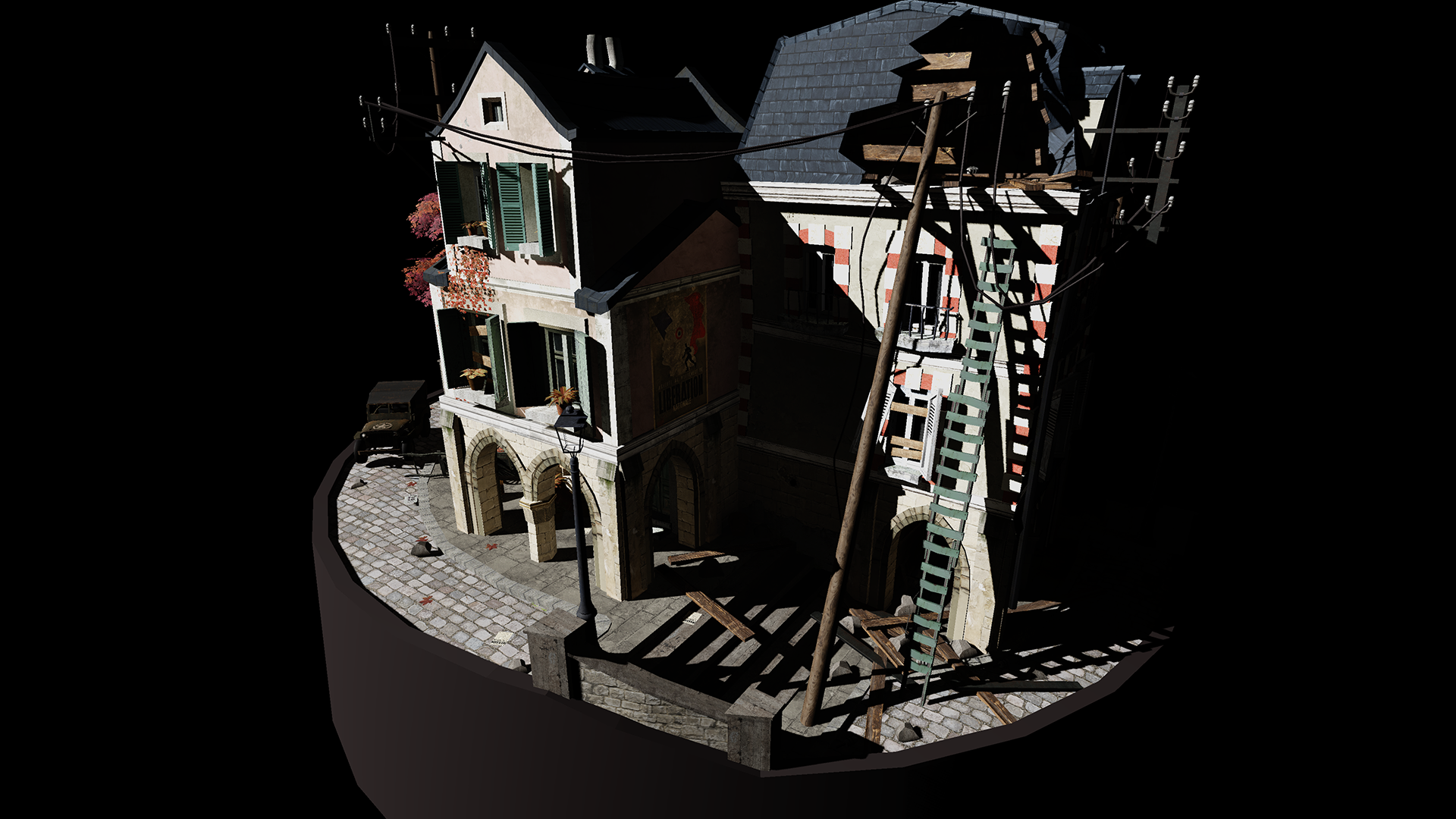
To be totally transparent about the cover image of this article. The given time for the project did not allow me to implement localized tone mapping. To be able to showcase an image with visible details in both the highlight and shadows I had to simulate the tone mapping through photoshop by blending a high and low exposure image based on luminance values. All images used are showed below: